
This document is one of More SageMath Tutorials. You may edit it on github. \(\def\NN{\mathbb{N}}\) \(\def\ZZ{\mathbb{Z}}\) \(\def\QQ{\mathbb{Q}}\) \(\def\RR{\mathbb{R}}\) \(\def\CC{\mathbb{C}}\)
Start here!
About SageMath and this document
SageMath (Sage for short) is a general
purpose computational mathematics system developed by a worldwide
community of hundreds of researchers, teachers and engineers. It’s
based on the Python programming language and includes GAP, PARI/GP,
Singular, and dozens of other specialized libraries.
This live document will guide you through the first steps of using Sage, and provide pointers to explore and learn further.
In the following, we will be assuming that you are reading this
document as a Jupyter notebook (Jupyter is the primary user interface
for Sage). If instead you are reading this document as a web page, you can click
on Run on mybinder.org to get access to the notebook online. If
you have Sage already installed on your machine, you may instead
download this page As Jupyter notebook. If you just want to try
out a few things, you may also just click the Activate button on
the upper right corner to play with the examples.
Todo
- credits on the many sources of inspiration
Entering, editing, and evaluating input
A first calculation
Sage can be used as a pocket calculator: you type in some expression
to be calculated, Sage evaluates it, and prints the result; and
repeat. This is called the Read-Eval-Print-Loop. In the Jupyter
notebook, you type the expression in an input cell, or code
cell. This is the rectangle below this paragraph containing \(1+1\)
(if instead you see sage: 1+1, you are reading this document as a
web page and won’t be able to play with the examples). Click on the
cell to select it, and press shift-enter to evaluate it:
sage: 1 + 1
2
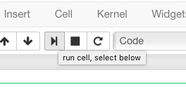
You may instead click the play button in the tool bar or use the
Cell menu:
Sage prints out its response in an output cell just below the
input cell (that’s the 2, so Sage confirms that \(1+1=2\)).
Click again in the cell, replace \(1+1\) by \(2+2\),
and evaluate it. Notice how much quicker it is now? That’s because a
Sage process had to be started the first time, and then stayed ready.
Congratulations, you have done your first calculations with Sage.
Using the Jupyter Notebook
Now take some time to explore the Help menu. We specifically
recommend taking the User Interface Tour, and coming back to
Keyboard shortcuts every now and then to get fast at Jupyter.
The Jupyter developers also maintain a tutorial notebook
which you may find useful.
For now we just review the basics. Use the menu item Insert ->
Insert Cell Below to create a new input cell below this paragraph,
then calculate any simple expression of your liking.
You can move around and edit any cell by clicking in it. Go back and change your \(2+2\) above to \(3+3\) and re-evaluate it.
You can also edit any text cell by double clicking on it. Try it now! The text you see is using the Markdown markup language. Do some changes to the text, and evaluate it again to rerender it. Markdown supports a fair amount of basic formatting, such as bold, underline, basic lists, and so forth. Thanks to the TeX rendering engine MathJax, you may embed mathematical formulae such as $sin(x) - y^3$ just like with LaTeX. It can be fun to type in fairly complicated math, like this:
If you mess everything up, you can use the menu Kernel ->
Restart to restart Sage. You can also use the menu File -> Save and
Checkpoint to save notebook, and File -> Revert to Checkpoint -> ...
to reset to any previously saved version.
More interactions
We are now done with basic interaction with Sage. Much richer
interactions are possible thanks to Jupyter’s interactive widgets.
That will be the topic for a later tutorial; here is just a teaser for
now. Try clicking on the sliders to illustrate multiplication below.
Also, you can try changing the slider ranges to something different by
editing the input cell (make sure to also change xmax, ymax):
sage: @interact                                # not tested
....: def f(n=(1 .. 15), m=(1 .. 15)):
....:     print("n * m = {} = {}".format(n * m, factor(n * m)))
....:     P = polygon([(0, 0), (0, n), (m, n), (m, 0)])
....:     P.show(aspect_ratio=1, gridlines='minor', figsize=[3, 3], xmax=14, ymax=14)
A brief tour
Sage covers many areas of mathematics:
2D/3D Graphics, Categories, Basic Rings and Fields: Integers and Rational Numbers, Real and Complex Numbers, Finite Rings and Fields, Polynomials, Formal Power Series, p-Adic Numbers, Quaternion Algebras, Linear Algebra: Matrices and Spaces of Matrices, Vectors and Modules, Tensors on Free Modules of Finite Rank, Calculus and Analysis: Symbolic Calculus, Mathematical Constants, Elementary and Special Functions, Asymptotic Expansions, Numerical Optimization, Probability and Statistics, Probability , Statistics, Quantitative Finance, Mathematical Structures: Sets, Monoids, Groups, Semirings, Rings, Algebras, Discrete Mathematics Combinatorics, Graph Theory, Quivers, Matroid Theory, Discrete Dynamics, Coding Theory, Cryptography, Game Theory, Symbolic Logic, SAT solvers, Geometry and Topology: Combinatorial and Discrete Geometry, Hyperbolic Geometry, Cell Complexes and their Homology, Differential Forms, Manifolds, Parametrized Surfaces, Knot Theory, Number Fields and Function Fields, Number Theory: Diophantine approximation, Quadratic Forms, L-Functions, Arithmetic Subgroups of \(SL_2(Z)\), General Hecke Algebras and Hecke Modules, Modular Symbols, Modular Forms, Modular Forms for Hecke Triangle Groups, Modular Abelian Varieties, Algebraic and Arithmetic Geometry: Schemes, Plane, Elliptic and Hyperelliptic Curves, Databases, Games
We now engage in a brief tour.
Todo
- Better formatting of the above list of areas, with links to relevant pieces of the documentation.
- Insert more striking examples (including Sage-Manifolds!)
- Insert Read More links
Calculus
sage: %display latex
sage: x,y = var('x,y')
sage: f = (cos(pi/4-x)-tan(x)) / (1-sin(pi/4 + x)); f
-(cos(1/4*pi - x) - tan(x))/(sin(1/4*pi + x) - 1)
sage: limit(f, x = pi/4, dir='minus')
+Infinity

sage: solve([x^2+y^2 == 1, y^2 == x^3 + x + 1], x, y)
[[x == -1/2*I*sqrt(3) - 1/2, y == -sqrt(-1/2*I*sqrt(3) + 3/2)],
 [x == -1/2*I*sqrt(3) - 1/2, y == sqrt(-1/2*I*sqrt(3) + 3/2)],
 [x == 1/2*I*sqrt(3) - 1/2, y == -sqrt(1/2*I*sqrt(3) + 3/2)],
 [x == 1/2*I*sqrt(3) - 1/2, y == sqrt(1/2*I*sqrt(3) + 3/2)],
 [x == 0, y == -1], [x == 0, y == 1]]

sage: plot3d(sin(pi*sqrt(x^2+y^2)) / sqrt(x^2+y^2), (x,-5,5), (y,-5,5), viewer="threejs")
Graphics3d Object

sage: contour_plot(y^2 + 1 - x^3 - x, (x,-pi,pi), (y,-pi,pi),
....:              contours=[-8,-4,0,4,8], colorbar=True)
Graphics object consisting of 1 graphics primitive
Algebra
sage: factor(x^100 - 1)
(x^40 - x^30 + x^20 - x^10 + 1)*(x^20 + x^15 + x^10 + x^5 + 1)*(x^20 - x^15 + x^10 - x^5 + 1)*(x^8 - x^6 + x^4 - x^2 + 1)*(x^4 + x^3 + x^2 + x + 1)*(x^4 - x^3 + x^2 - x + 1)*(x^2 + 1)*(x + 1)*(x - 1)

sage: p = 54*x^4+36*x^3-102*x^2-72*x-12
sage: p.factor()
6*(x^2 - 2)*(3*x + 1)^2

sage: for K in [ZZ, QQ, ComplexField(16), QQ[sqrt(2)], GF(5)]:
....:     print(K, ":"); print(K['x'](p).factor())
Integer Ring :
2 * 3 * (3*x + 1)^2 * (x^2 - 2)
Rational Field :
(54) * (x + 1/3)^2 * (x^2 - 2)
Complex Field with 16 bits of precision :
(54.00) * (x - 1.414) * (x + 0.3333)^2 * (x + 1.414)
Number Field in sqrt2 with defining polynomial x^2 - 2 :
(54) * (x - sqrt2) * (x + sqrt2) * (x + 1/3)^2
Finite Field of size 5 :
(4) * (x + 2)^2 * (x^2 + 3)

sage: ZZ.category()
Join of Category of euclidean domains and Category of infinite enumerated sets and Category of metric spaces

sage: sorted( ZZ.category().axioms() )
['AdditiveAssociative', 'AdditiveCommutative', 'AdditiveInverse', 'AdditiveUnital',
 'Associative', 'Commutative', 'Distributive',
 'Enumerated', 'Infinite',
 'NoZeroDivisors',
 'Unital']
Linear algebra
sage: A = matrix(GF(7), 4, [5,5,4,3,0,3,3,4,0,1,5,4,6,0,6,3]); A
[5 5 4 3]
[0 3 3 4]
[0 1 5 4]
[6 0 6 3]

sage: P = A.characteristic_polynomial(); P
x^4 + 5*x^3 + 6*x + 2

sage: P(A)
[0 0 0 0]
[0 0 0 0]
[0 0 0 0]
[0 0 0 0]

sage: A.eigenspaces_left()
[
(4, Vector space of degree 4 and dimension 1 over Finite Field of size 7
User basis matrix:
[1 4 6 1]),
(1, Vector space of degree 4 and dimension 1 over Finite Field of size 7
User basis matrix:
[1 3 3 4]),
(2, Vector space of degree 4 and dimension 2 over Finite Field of size 7
User basis matrix:
[1 0 2 3]
[0 1 6 0])
]
Computing the rank of a large sparse matrix:
sage: M = random_matrix(GF(7), 10000, sparse=True, density=3/10000)
sage: M.rank()                        # random
9263
Geometry
sage: polytopes.truncated_icosidodecahedron().plot(viewer="threejs")
Graphics3d Object
Programming and plotting
sage: n, l, x, y = 10000, 1, 0, 0
sage: p = [[0, 0]]
sage: for k in range(n):
....:     theta = (2 * pi * random()).n(digits=5)
....:     x, y = x + l * cos(theta), y + l * sin(theta)
....:     p.append([x, y])
sage: g = line(p, thickness=.4) + line([p[n], [0, 0]], color='red', thickness=2)
sage: g.show(aspect_ratio=1)
Interactive plots
sage: x = var('x')
sage: @interact                                # not tested
....: def g(f=x*sin(1/x),
....:       c=slider(-1, 1, .01, default=-.5),
....:       n=(1..30),
....:       xinterval=range_slider(-1, 1, .1, default=(-8,8), label="x-interval"),
....:       yinterval=range_slider(-1, 1, .1, default=(-3,3), label="y-interval")):
....:     x0 = c
....:     degree = n
....:     xmin,xmax = xinterval
....:     ymin,ymax = yinterval
....:     p   = plot(f, xmin, xmax, thickness=4)
....:     dot = point((x0,f(x=x0)),pointsize=80,rgbcolor=(1,0,0))
....:     ft = f.taylor(x,x0,degree)
....:     pt = plot(ft, xmin, xmax, color='red', thickness=2, fill=f)
....:     show(dot + p + pt, ymin=ymin, ymax=ymax, xmin=xmin, xmax=xmax)
....:     html('$f(x)\;=\;%s$'%latex(f))
....:     html('$P_{%s}(x)\;=\;%s+R_{%s}(x)$'%(degree,latex(ft),degree))
Graph Theory
Coloring graphs:
sage: g = graphs.PetersenGraph(); g
Petersen graph: Graph on 10 vertices
sage: g.plot(partition=g.coloring())
Graphics object consisting of 26 graphics primitives
Combinatorics
Fast counting:
sage: Partitions(100000).cardinality()
27493510569775696512677516320986352688173429315980054758203125984302147328114964173055050741660736621590157844774296248940493063070200461792764493033510116079342457190155718943509725312466108452006369558934464248716828789832182345009262853831404597021307130674510624419227311238999702284408609370935531629697851569569892196108480158600569421098519
Playing poker:
sage: Suits   = Set(["Hearts", "Diamonds", "Spades", "Clubs"])
sage: Values  = Set([2, 3, 4, 5, 6, 7, 8, 9, 10, "Jack", "Queen", "King", "Ace"])
sage: Cards   = cartesian_product([Values, Suits])
sage: Hands   = Subsets(Cards, 5)
sage: Hands.random_element()                        # random
{(5, 'Pique'), (4, 'Coeur'), (8, 'Trefle'), ('As', 'Trefle'), (10, 'Carreau')}
sage: Hands.cardinality()
2598960
Algebraic Combinatorics
Drawing an affine root systems:
sage: L = RootSystem(["G", 2, 1]).ambient_space()
sage: p = L.plot(affine=False, level=1)
sage: p.show(aspect_ratio=[1, 1, 2], frame=False)
Number Theory
sage: E = EllipticCurve('389a')
sage: plot(E, thickness=3)
Graphics object consisting of 2 graphics primitives
Games
Sudoku solver:
sage: S = Sudoku('5...8..49...5...3..673....115..........2.8..........187....415..3...2...49..5...3'); S
+-----+-----+-----+
|5    |  8  |  4 9|
|     |5    |  3  |
|  6 7|3    |    1|
+-----+-----+-----+
|1 5  |     |     |
|     |2   8|     |
|     |     |  1 8|
+-----+-----+-----+
|7    |    4|1 5  |
|  3  |    2|     |
|4 9  |  5  |    3|
+-----+-----+-----+

sage: list(S.solve())
[+-----+-----+-----+
 |5 1 3|6 8 7|2 4 9|
 |8 4 9|5 2 1|6 3 7|
 |2 6 7|3 4 9|5 8 1|
 +-----+-----+-----+
 |1 5 8|4 6 3|9 7 2|
 |9 7 4|2 1 8|3 6 5|
 |3 2 6|7 9 5|4 1 8|
 +-----+-----+-----+
 |7 8 2|9 3 4|1 5 6|
 |6 3 5|1 7 2|8 9 4|
 |4 9 1|8 5 6|7 2 3|
 +-----+-----+-----+]
Help system
We review the three main ways to get help in Sage:
- navigating through the documentation,
- tab-completion,
- contextual help.
Completion and contextual documentation
Start typing something and press the Tab key. The interface tries to
complete it with a command name. If there is more than one completion, then
they are all presented to you. Remember that Sage is case sensitive, i.e. it
differentiates upper case from lower case. Hence the Tab completion of
klein won’t show you the KleinFourGroup command that builds the group
\(\ZZ/2 \times \ZZ/2\) as a permutation group. Try pressing the Tab
key in the following cells:
sage: klein

sage: Klein
To see documentation and examples for a command, type a question mark
? at the end of the command name and evaluate the cell:
sage: KleinFourGroup?
sage:
Exercise A
What is the largest prime factor of \(600851475143\)?
sage: factor?
sage:
Digression: assignments and methods
In the above manipulations we did not store any data for
later use. This can be done in Sage with the = symbol as in:
sage: a = 3
sage: b = 2
sage: a + b
5
This can be understood as Sage evaluating the expression to the right
of the = sign and creating the appropriate object, and then
associating that object with a label, given by the left-hand side (see
the foreword of Tutorial: Objects and Classes in Python and Sage for
details). Multiple assignments can be done at once:
sage: a, b = 2, 3
sage: a
2
sage: b
3
This allows us to swap the values of two variables directly:
sage: a, b = 2, 3
sage: a, b = b, a
sage: a, b
(3, 2)
We can also assign a common value to several variables simultaneously:
sage: c = d = 1
sage: c, d
(1, 1)
sage: d = 2
sage: c, d
(1, 2)
Note that when we use the word variable in the computer-science sense we mean “a label attached to some data stored by Sage”. Once an object is created, some methods apply to it. This means functions but instead of writing f(my_object) you write my_object.f():
sage: p = 17
sage: p.is_prime()
True
See Tutorial: Objects and Classes in Python and Sage for details.
Method discovery with tab-completion
Todo
Replace the examples below by less specialized ones
To know all methods of an object you can once more use tab-completion.
Write the name of the object followed by a dot and then press Tab:
sage: a.
Exercise B
Create the permutation 51324 and assign it to the variable p.
sage: Permutation?
sage:
What is the inverse of p?
sage: p.inv

sage:
Does p have the pattern 123? What about 1234? And 312? (even if you don’t
know what a pattern is, you should be able to find a command that does this).
sage: p.pat

sage:
Exercises
Linear algebra
Exercise C
Use the matrix() command to create the following matrix.
sage: matrix?
sage:
Then, using methods of the matrix,
- Compute the determinant of the matrix.
- Compute the echelon form of the matrix.
- Compute the eigenvalues of the matrix.
- Compute the kernel of the matrix.
- Compute the LLL decomposition of the matrix (and lookup the documentation for what LLL is if needed!)
sage:

sage:
Now that you know how to access the different methods of matrices,
- Create the vector \(v = (1, -1, -1, 1)\).
- Compute the two products: \(M \cdot v\) and \(v \cdot M\). What mathematically borderline operation is Sage doing implicitly?
sage: vector?
sage:
Note
Vectors in Sage can be used as row vectors or column vectors.
A method such as eigenspaces might not
return what you expect, so it is best to specify eigenspaces_left or
eigenspaces_right instead. Same thing for kernel (left_kernel or
right_kernel), and so on.
Plotting
The plot() command allows you to draw plots of functions. Recall
that you can access the documentation by pressing the Tab key
after writing plot? in a cell:
sage: plot?
sage:
Here is a simple example:
sage: var('x')   # make sure x is a symbolic variable
x
sage: plot(sin(x^2), (x, 0, 10))
Graphics object consisting of 1 graphics primitive
Here is a more complicated plot. Try to change every single input to the plot command in some way, evaluating to see what happens:
sage: P = plot(sin(x^2), (x, -2, 2), rgbcolor=(0.8, 0, 0.2), thickness=3, linestyle='--', fill='axis')
sage: show(P, gridlines=True)
Above we used the show() command to show a plot after it was created. You can
also use P.show instead:
sage: P.show(gridlines=True)
Try putting the cursor right after P.show( and pressing Tab to get a list of
the options for how you can change the values of the given inputs.
sage: P.show(
Plotting multiple functions at once is as easy as adding the plots together:
sage: P1 = plot(sin(x), (x, 0, 2*pi))
sage: P2 = plot(cos(x), (x, 0, 2*pi), rgbcolor='red')
sage: P1 + P2
Graphics object consisting of 2 graphics primitives
Symbolic Expressions
Here is an example of a symbolic function:
sage: f(x) = x^4 - 8*x^2 - 3*x + 2
sage: f(x)
x^4 - 8*x^2 - 3*x + 2

sage: f(-3)
20
This is an example of a function in the mathematical variable \(x\). When Sage starts, it defines the symbol \(x\) to be a mathematical variable. If you want to use other symbols for variables, you must define them first:
sage: x^2
x^2
sage: u + v
Traceback (most recent call last):
...
NameError: name 'u' is not defined

sage: var('u v')
(u, v)
sage: u + v
u + v
Still, it is possible to define symbolic functions without first defining their variables:
sage: f(w) = w^2
sage: f(3)
9
In this case those variables are defined implicitly:
sage: w
w
Exercise D
Define the symbolic function \(f(x) = x \sin(x^2)\). Plot \(f\) on the
domain \([-3, 3]\) and color it red. Use the find_root() method to
numerically approximate the root of \(f\) on the interval \([1, 2]\):
sage:
Compute the tangent line to \(f\) at \(x = 1\):
sage:
Plot \(f\) and the tangent line to \(f\) at \(x = 1\) in one image:
sage:
Exercise E (Advanced)
Solve the following equation for \(y\):
There are two solutions, take the one for which \(\lim_{x\to0} y(x) = 1\). (Don’t forget to create the variables \(x\) and \(y\)!).
sage:
Expand \(y\) as a truncated Taylor series around \(0\) containing \(n = 10\) terms.
sage:
Do you recognize the coefficients of the Taylor series expansion? You might
want to use the On-Line Encyclopedia of Integer Sequences, or better yet, Sage’s class OEIS which
queries the encyclopedia:
sage: oeis?
sage:
Congratulations for completing your first Sage tutorial!
Exploring further
Accessing Sage
The Sage cell service lets you evaluate individual Sage commands.
In general, Sage computations can be embedded in any web page using Thebelab or the Sage-cell server.
Binder is a service that lets you run Jupyter online on top of an arbitrary software stack. Sessions are free, anonymous, and temporary. You can use one of the existing repositories, or create your own.
Todo
add links about both
Cocalc (Collaborative Calculation in the Cloud) is an online service that gives access to a wealth of computational systems, including Sage, with extra goodies for teaching. It’s free for basic usage.
JupyterHub lets you (or your institution or …) deploy a multi-user Jupyter service.
The Sage Debian Live USB key let’s you run Linux with Sage and many other goodies on your computer without having to install them.
Sage can be installed on most major operating systems (Linux, macOS, Windows), through usual package managers or installers, or by compiling from source.
Ways to use Sage
There are many ways beyond the Jupyter Notebook to use Sage: interactive command line, program scripts, … See the Sage tutorial.
Note
Sage used to have its own legacy notebook system, which has been phased out in favor of Jupyter. If you have old notebooks, here is how to migrate them.
Resources
- Sage’s web page: https://www.sagemath.org
- Ask Sage: https://ask.sagemath.org
- Bug Tracker: https://trac.sagemath.org
- The open book Computational Mathematics with Sage (originally written in French; also translated in German)
- Sage’s main tutorial
- Sage’s official thematic tutorials
- More Sage tutorials
- Sage’s quick reference cards